Compute Post Simulation Average

This week, we're highlighting a newly added command: compute post simulation average. This command was designed to simplify coupling PEST (Parameter Estimation) with HydroGeoSphere (HGS) by extracting average values of simulated quantities over a specified time interval and storing them in a file that PEST can easily read.

Executed at the end of an HGS simulation, the compute post simulation average command works with time series output such as observation points, hydrographs, and more. The command structure allows you to specify the quantities you want to average, along with the time intervals for each calculation. This addition is particularly useful for those working with PEST or those requiring post-simulation averaging of quantities for further analysis.

---

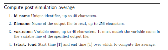
Figure 1: Command description

This week we are looking at a recently added command: compute post simulation average. This command was added to HGS to make it easier to couple PEST to HGS by extracting average values of simulated quantities over a specified time interval, and storing them in a file that is easy for PEST to read. This command is executed at the completion of an HGS simulation and works with time series output from the simulation (i.e., observation point, hydrograph, etc.). The input structure for this command is described in Figure 1.

When invoking this command, the user will need to provide four additional lines of input instructions. The first line provides a unique identifier for the new variable which will be written to file by the compute post simulation average command (id_name). The second line provides the name of output file which contains the data which you would like to average (filename). In the third line you will list the name of the variable which you would like to average (var_name), and must match the variable name listed in the specified output file (i.e. filename). For example, observation point output files typically will include output variables for hydraulic head (“H”), pressure head (“P”), saturation (“S”), volumetric water content (“VWC”), etc. Each of these variable names (i.e. H, P, S, VWC) is a suitable input for var_name. Finally, the fourth line will list the start (tstart) and end time (tend) over which to compute the average.

We've included an example (click here to download) based on the Abdul Transport problem which has 4 average quantities being computed over different time intervals as follows:

      compute post simulation average
      head_1
      abdul_transo.observation_well_flow.point1.dat
      H
      0 3000

      compute post simulation average
      head_2
      abdul_transo.observation_well_flow.point1.dat
      H
      3000 6000

      compute post simulation average
      sat_1
      abdul_transo.observation_well_flow.point1.dat
      S
      0 3000

      compute post simulation average
      conc_1
      abdul_transo.observation_well_conc.point1.Rain.dat
      C
      0 6000

Figure 2: Compute Post Simulation Average example output

Output is written to prefixo.avg_val_summary.dat as shown in Figure 2. Please note that unlike most output files, this file will only be created after the simulation is complete.

The command may be called any number of times, where each call adds a new line to the generated output file. The output variables in the resulting output file include “ID” (corresponding to the id_name), “Column #” (which indicates the column of the original source data within the defined output file, i.e. filename), “Column Header” (which corresponds to var_name), “T_start” and “T_end” (which correspond to Tstart and Tend, respectively), and finally the “Average_value” variable which corresponds to actual average value of the defined variable over the defined time period.