

Guide for New Users
We’re happy to provide all new users of HydroGeoSphere with a variety of training materials to help you understand how HydroGeoSphere works and how you can apply it to your own projects.
If you’re just starting out with HydroGeoSphere we recommend starting a free software trial, attending one of our free training sessions, and reviewing the comprehensive Intro to HGS tutorial.

Get Started with a Trial
Click the button below to request a temporary software license, and get in touch with our sales team for guidance.
Already Have a Software License?
Great — you’re ready to begin working with HydroGeoSphere. If you would like a guided introduction to the platform, we offer monthly training sessions. Click the training session button below to see upcoming events on our calendar.
For independent study we also recommend our interactive tutorial, which walks you through the full HGS workflow in detail and is an excellent starting point for new users. Click the button below to download a package of training materials to get started, including a comprehensive guidance document and a working HGS model.

Additional Resources
Discover supporting software solutions for HydroGeoSphere including AlgoMesh for triangular mesh generation, and ParaView/Tecplot for results visualization.

Visit our YouTube channel for more detailed instructional videos focused on different aspects of the HydroGeoShere workflow. We have training videos on everything from conceptual modelling to results visualization.
Visit the Aquanty blog for short-form HGS tutorials. These tutorials provide quick introductions to the many features offered by HGS, including advanced boundary conditions, troubleshooting numerical errors and more.
-
![]()
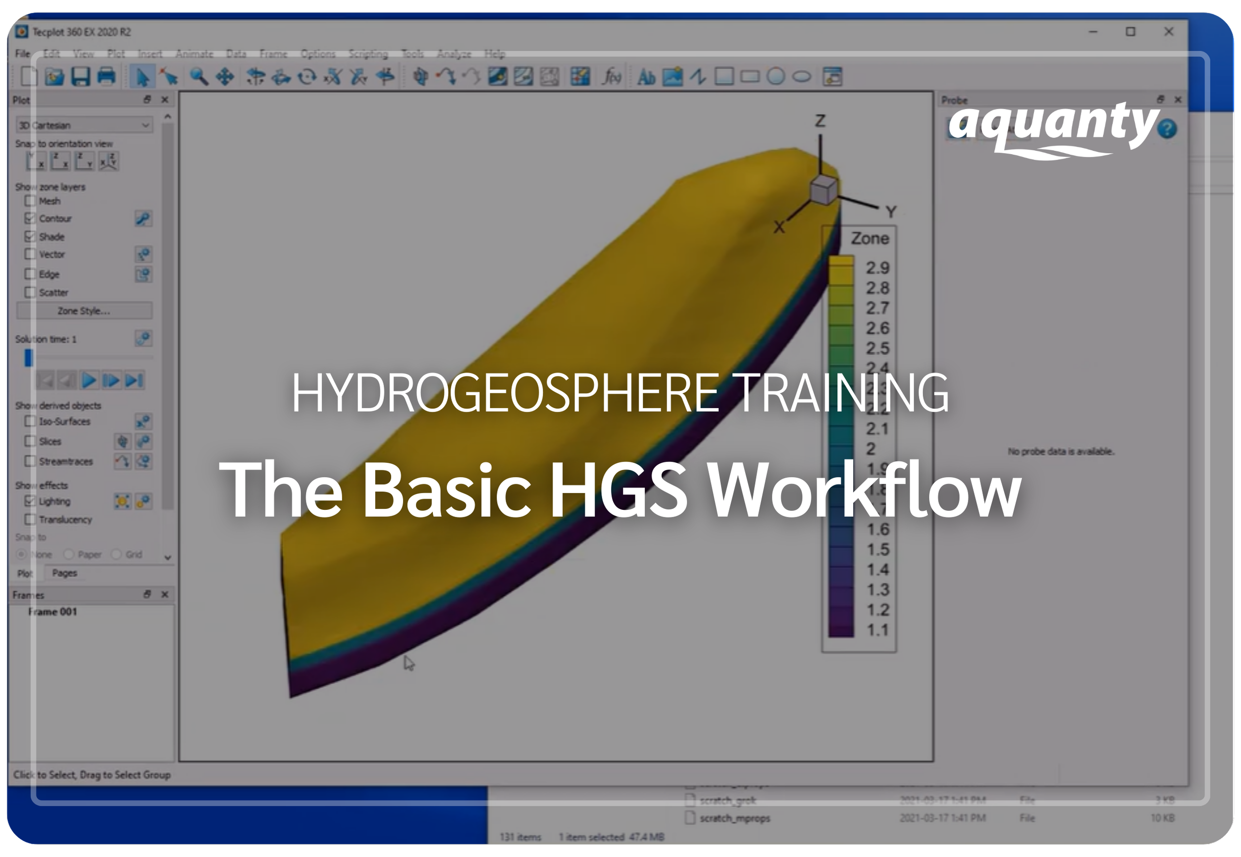
This short video demonstrates the essential workflow for building and running a HydroGeoSphere model— including a brief review of the HGS model input file and the process of running key HGS executables .
-
![A digital topographic map with green landmasses, blue river channels, and yellow-brown terrain outlines, overlaid with a white gear icon containing a water droplet and a hand.]()
This webinar introduces practical strategies for building high-quality, efficient HydroGeoSphere models— covering best practices for strong conceptual model development, boundary condition design, staged modeling, and numerical solver optimization to improve convergence and reduce runtimes.
-
![Scenic mountain landscape with snow-capped peaks reflecting in a calm lake, under a clear blue sky.]()
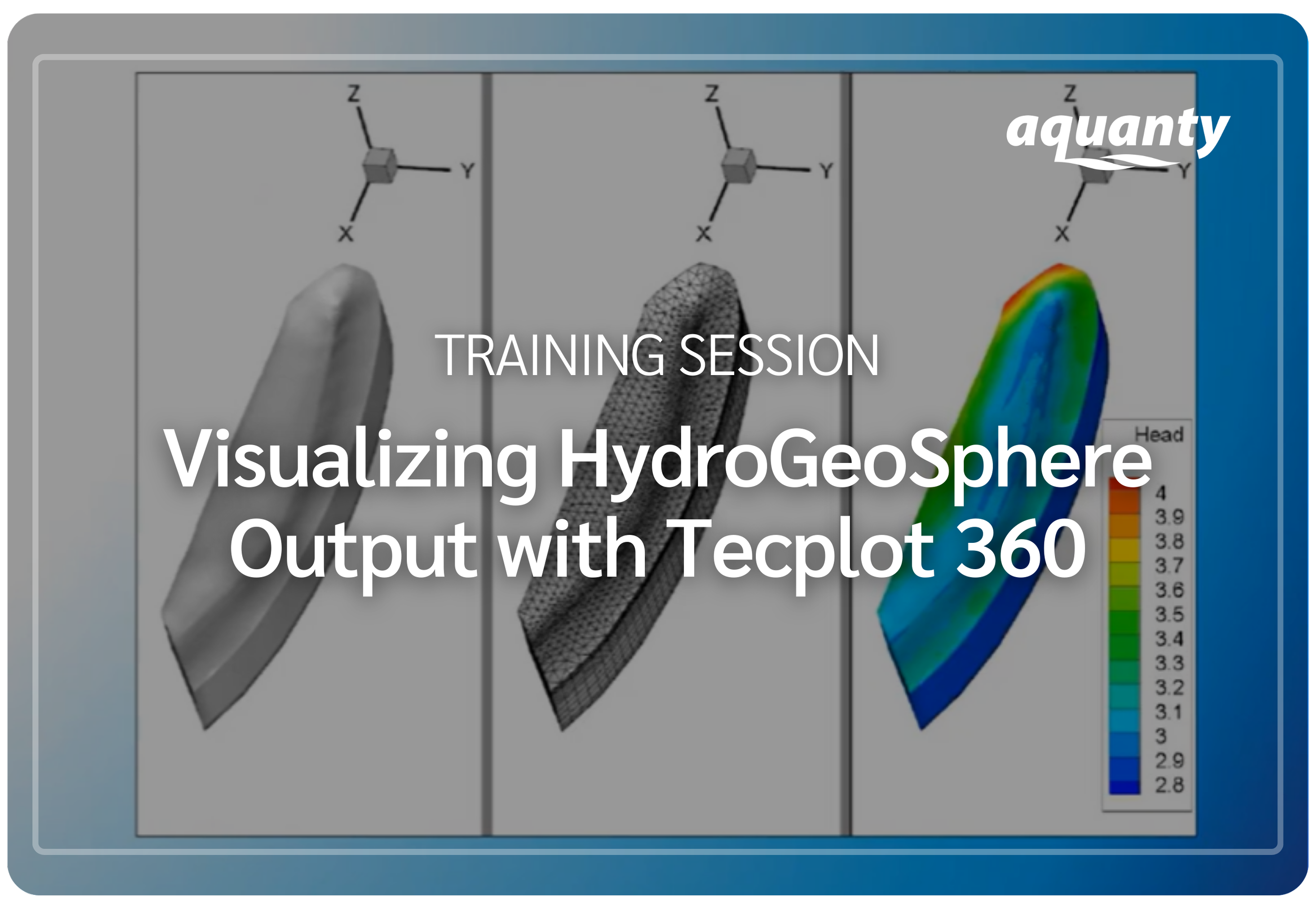
This video training session demonstrates how to visualize and communicate HydroGeoSphere model results using Tecplot 360— covering essential and advanced techniques for creating high-quality 2D/3D plots, images, and animations.
-
![]()
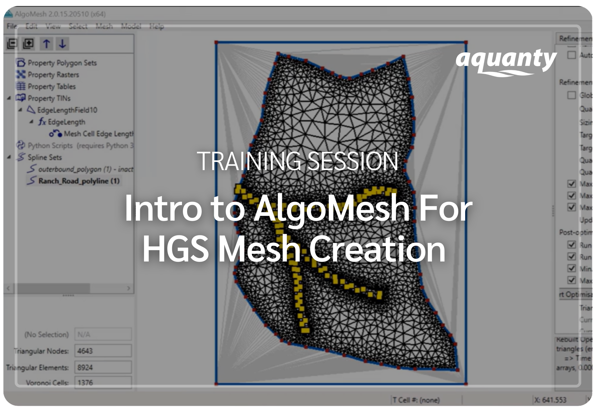
This recorded training session demonstrates how to generate high-quality unstructured meshes with AlgoMesh for use in HydroGeoSphere— covering the fundamentals of triangular finite element grids, mesh generation algorithms, and best practices for integrating real-world geometry into modeling workflows.
-
![Person in a red and black plaid shirt using a tablet in a wheat field, with a white leaf and checkmark eco-friendly logo overlay]()
This webinar demonstrates how to post-process and visualize HydroGeoSphere model outputs using HGS2VTU.exe—covering its core features, supported file formats, and time-series and resampling capabilities.
-
![A digital illustration featuring a cloud, a shield with a checkmark, and a network of connections, symbolizing cloud security and protection.]()
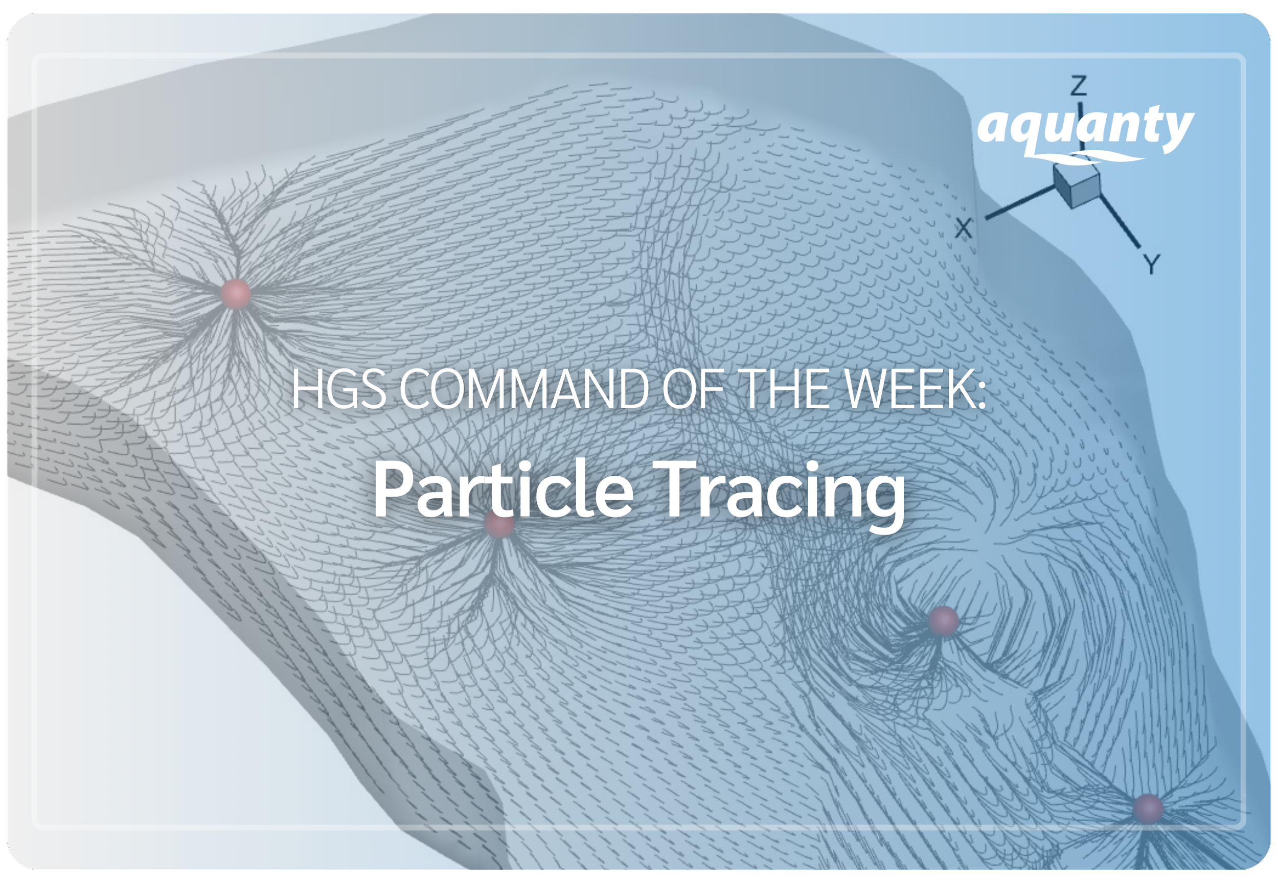
This tutorial introduces the particle tracing capabilities of HydroGeoSphere. Particle tracing allows users to track the movement of massless particles through the subsurface to visualize flow paths and transport dynamics.
-
![An aerial view of a coastal landscape with sandy beaches, grassy patches, and blue ocean waves, with a white overlay icon of a wave inside a circle.]()
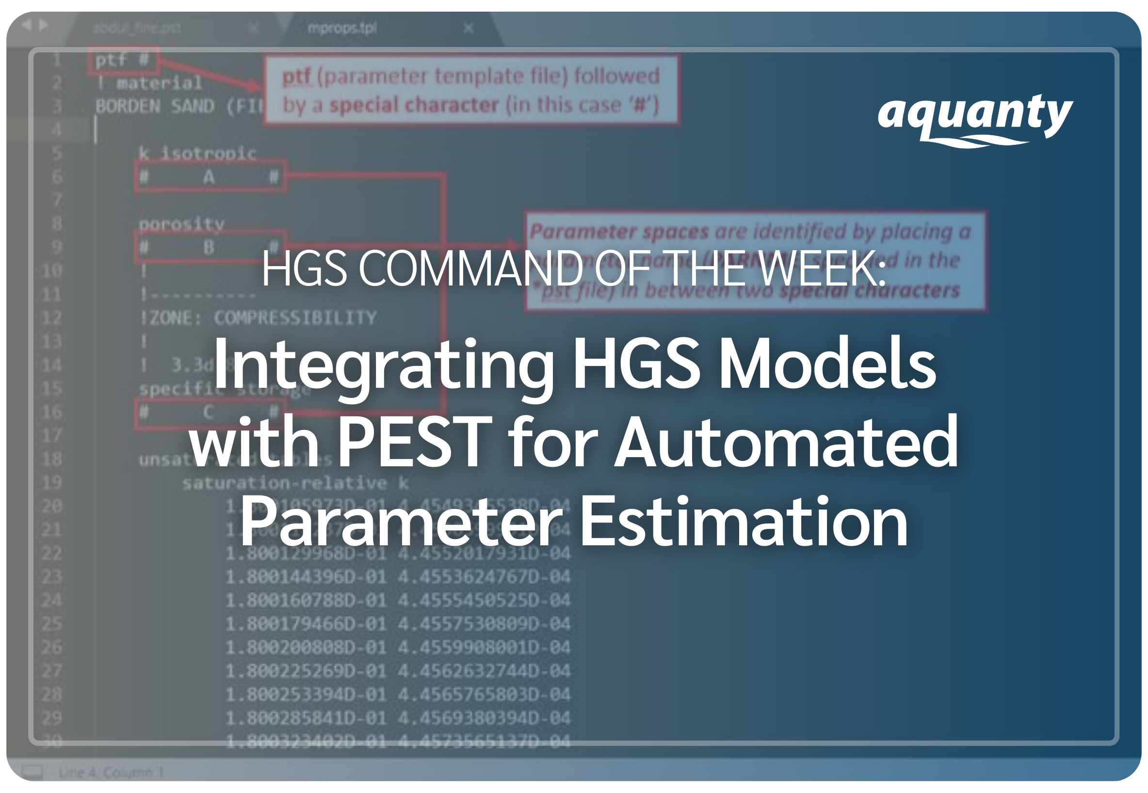
This tutorial introduces how to integrate PEST with HydroGeoSphere for automated parameter estimation and model calibration. Using the Abdul verification problem, it walks through PEST input file structure and shows how to run PEST to optimize HGS model parameters, with all required files provided.
-
![]()
This tutorial introduces the simple drain and makeup water boundary conditions in HydroGeoSphere to maintain a target head by allowing one-way inflow or outflow when thresholds are reached— an effective approach for modeling water management scenarios.
-
![]()
This tutorial explains how to use minimum layer thickness commands in HydroGeoSphere to enforce nodal elevation rules and prevent layer pinchouts when building model meshes, especially in complex geological systems.
-
![]()
This tutorial introduces the reservoir with spillway boundary condition in HydroGeoSphere, which improves reservoir simulations by enabling dynamic inflow and outflow control based on storage conditions— useful for modelling hydraulic water management systems.
-
![]()
This post explains how to use the debug.control file in HydroGeoSphere to adjust simulation performance in real time—allowing changes to convergence, time stepping, output, or pausing without restarting the model.
-
![]()
This post introduces the Map property from raster for chosen elements command in HydroGeoSphere (Rev. 2432), which simplifies assigning spatially variable properties from raster data with flexible mapping and smooth interpolation for heterogeneous models.
-
![]()
Explore how HydroGeoSphere is advancing integrated hydrologic modelling through real-world research applications. Visit our blog to discover the latest HGS Research Highlights and dive deeper into the science behind the work.
-
![]()
This post explains how to use Tecplot export commands in HydroGeoSphere to visualize model properties and structures without running a full simulation, helping users review setups and catch issues early.
-
![]()
Download the ‘Introductory Modules’ - a series of increasingly complex box models which can be reviewed to understand the structure of *.grok files. These are a great introduction to solute transport and discrete fracture flow.


Introducing The Graphical User Interface for HGS
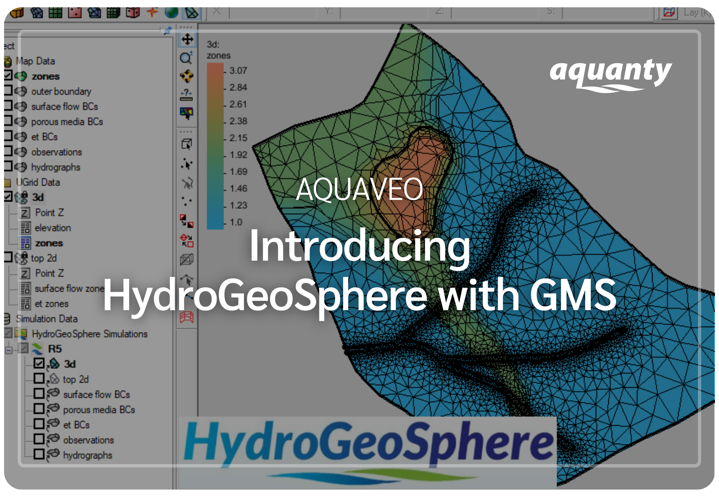
In February 2024, Aquanty announced the release of the HydroGeoSphere Interface in partnership with Aquaveo, bringing a graphical user interface (GUI) to the HGS modelling ecosystem through Groundwater Modeling System (GMS) v10.8.
This integration allows users to build fully integrated groundwater–surface water models using the HydroGeoSphere simulation engine directly within one of the world’s leading subsurface modelling platforms. Through the HGS Interface, GMS users can construct, parameterize, and visualize models using an intuitive graphical environment while maintaining access to the advanced physics-based capabilities that define HydroGeoSphere.
-
![]()
Through the HGS Interface for GMS, users can model watershed-scale processes including surface water, groundwater, and evapotranspiration, with expanded features planned for future releases.
-
![]()
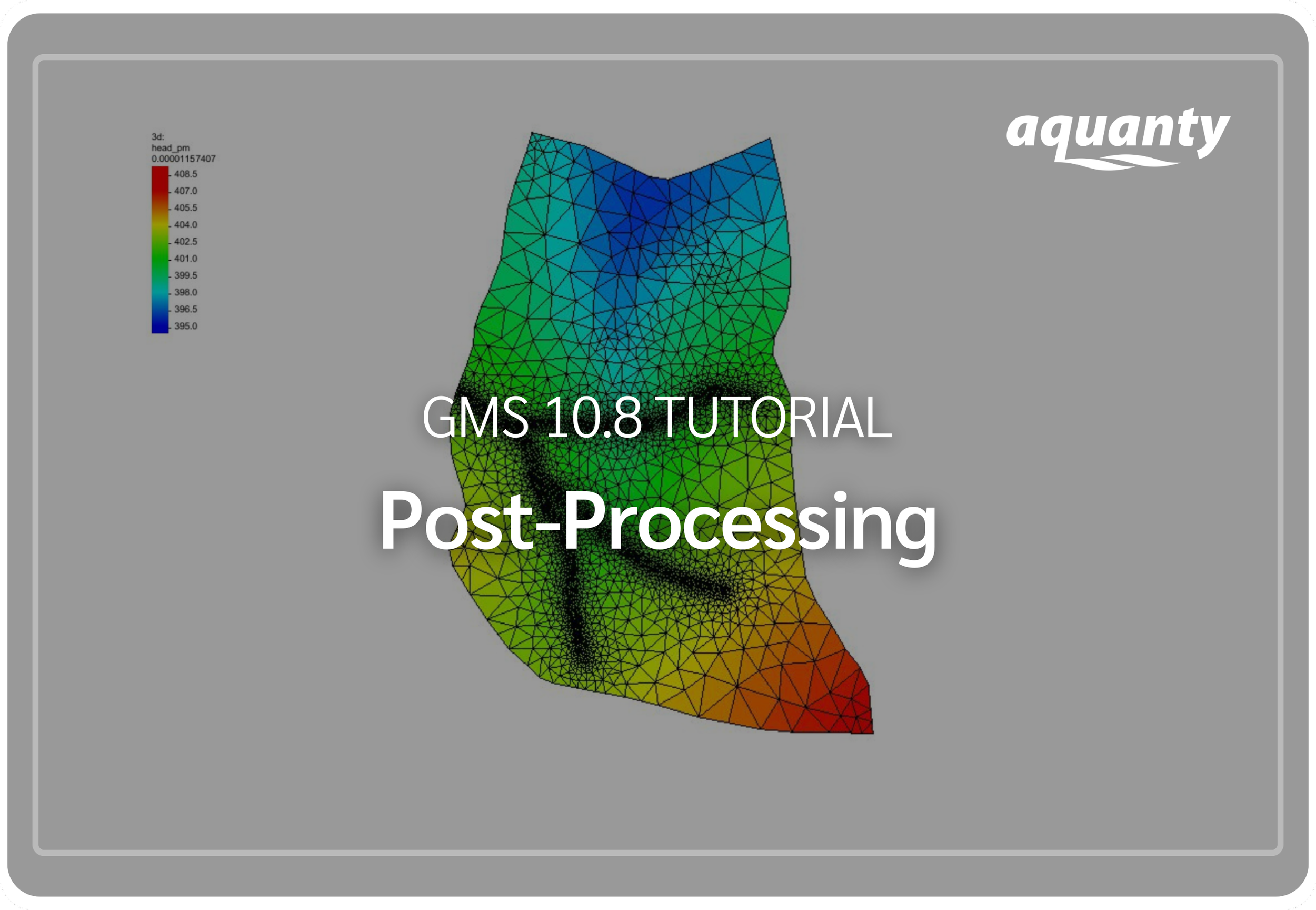
This tutorial demonstrates post-processing options for a HydroGeoSphere model in GMS. Click here to download the project files (.ZIP).
-
![]()
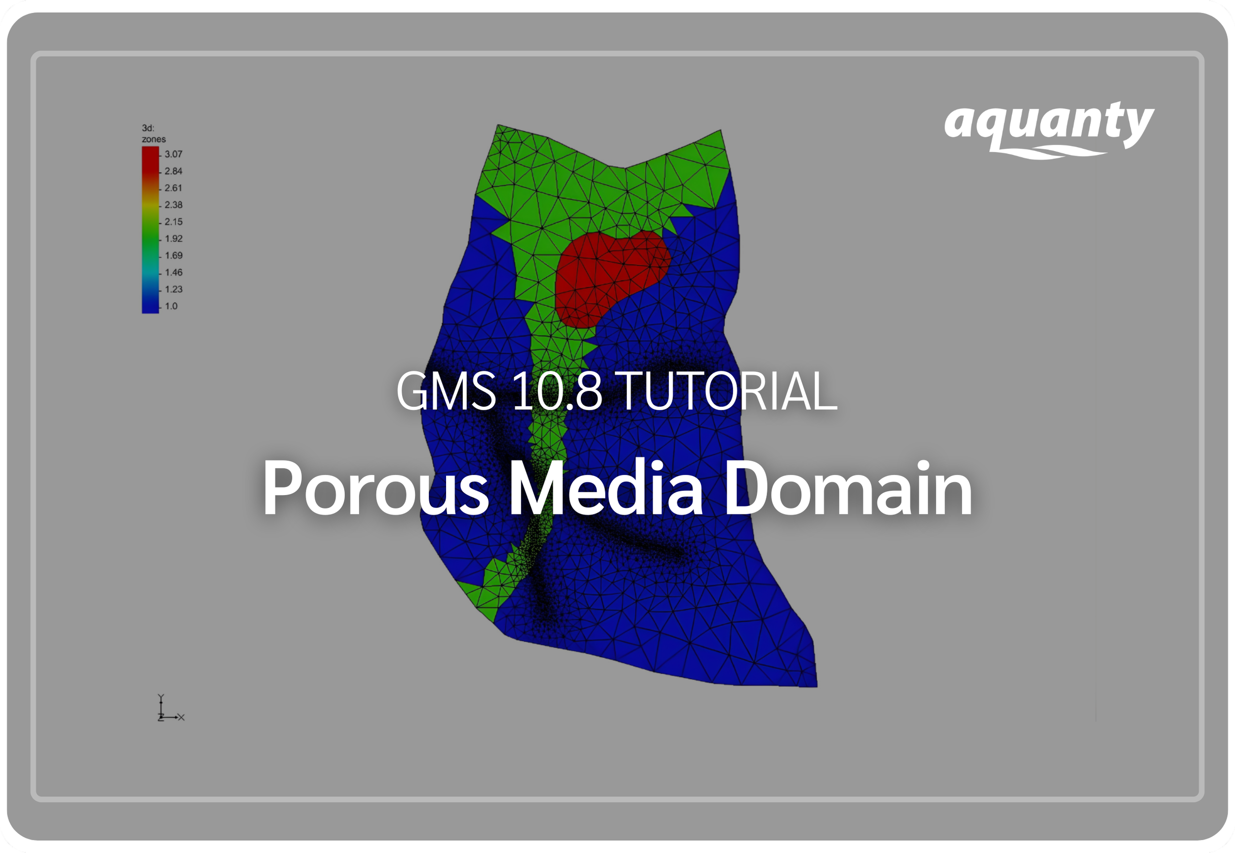
This tutorial demonstrates how to set up a HydroGeoSphere model with a porous media domain in GMS. Click here to download the project files (.ZIP).
-
![]()
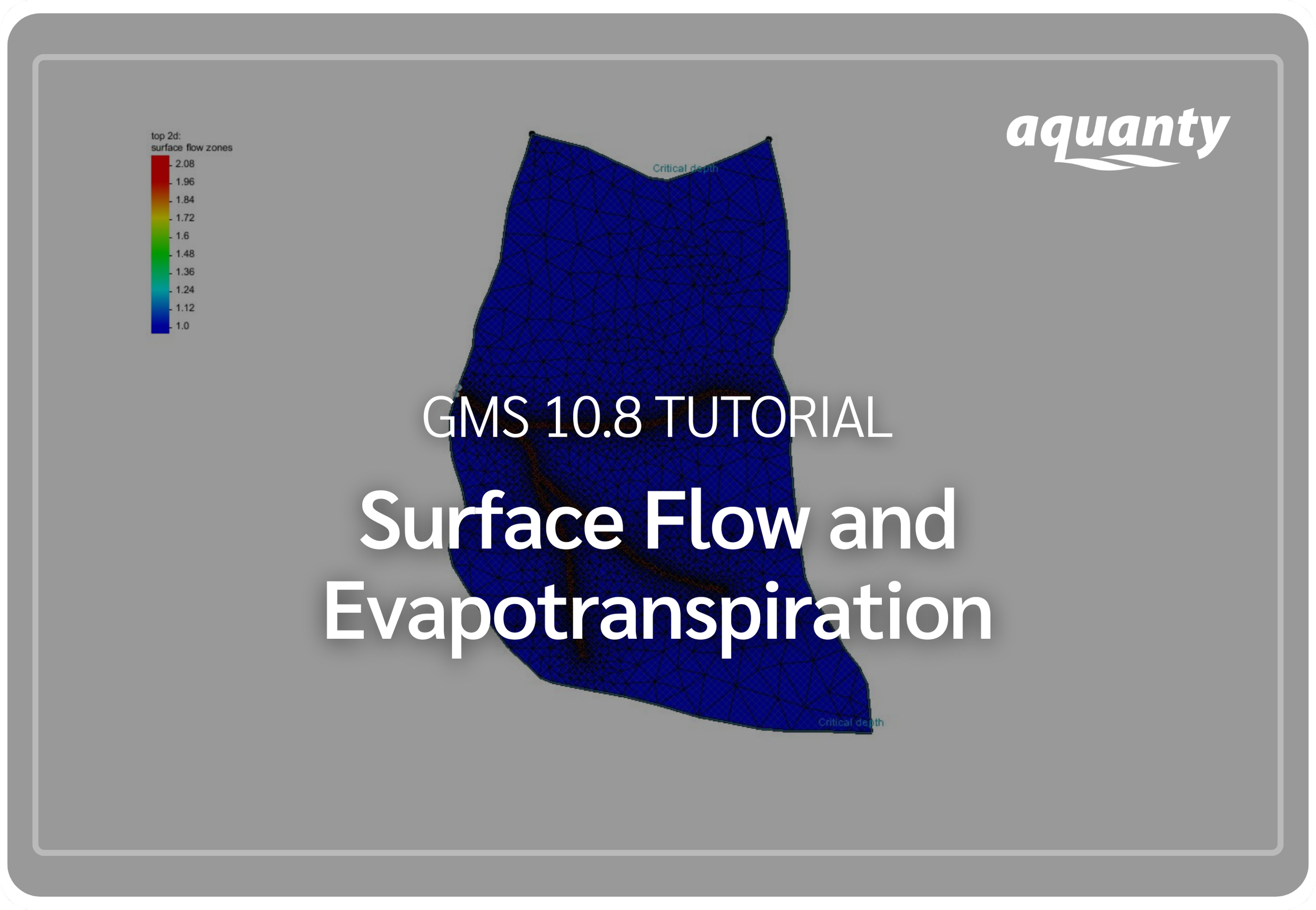
This tutorial demonstrates how to add surface flow and evapotranspiration to a HydroGeoSphere model in GMS. Click here to download the project files (.ZIP).
-
![]()
GMS 10.8 introduces a new HydroGeoSphere (HGS) interface, bringing Aquanty’s fully integrated, physics-based hydrologic model into GMS.
-
![]()
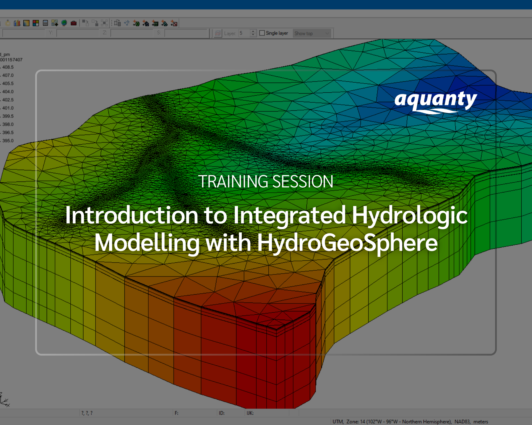
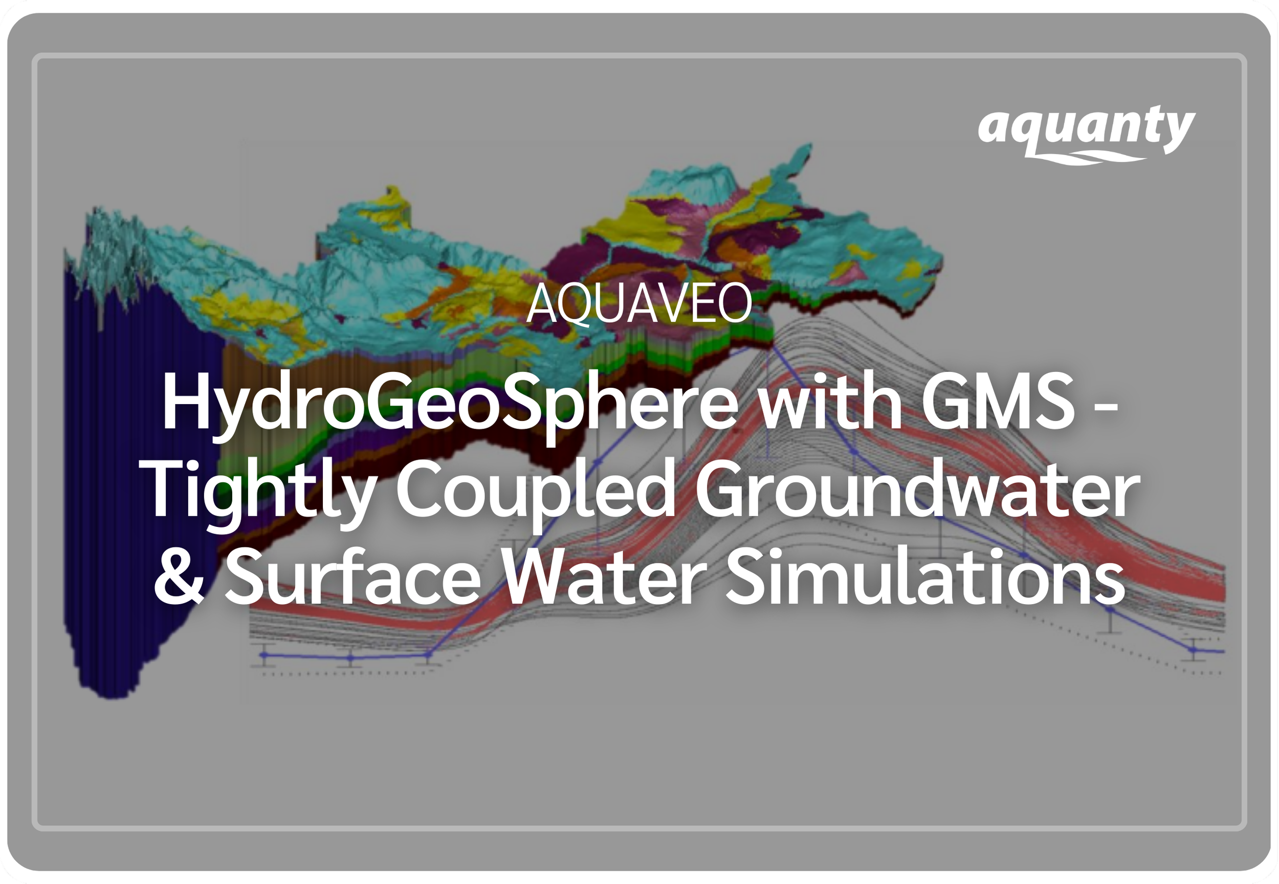
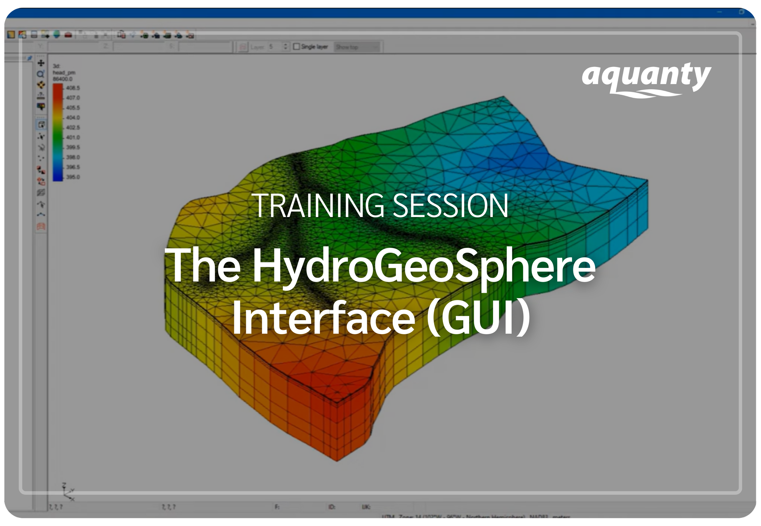
This webinar tutorial demonstrates how to build fully integrated groundwater–surface water models using the HydroGeoSphere Interface in GMS—showcasing the GUI, core flow and boundary condition tools, and a guided workflow developed in partnership with Aquaveo.
Join the HydroGeoSphere User Community
Connect with hydrologists, engineers, researchers, and practitioners from around the world who are using HydroGeoSphere to solve real-world water challenges. Our user community is a space to share insights, explore new features, discover case studies, and stay informed about software updates, webinars, and training opportunities.
Whether you’re just getting started or working on advanced integrated models, the HydroGeoSphere community is here to support your learning and help you get the most out of HGS.